This blog is the learning notes for preparing the preliminary exams of Queue theory, referring to Introduction to operations research
- Hillier, F. S., & Lieberman, G. J. (2015). Introduction to operations research. McGraw-Hill.
1. Introduction
These kinds ofproblems and the need to find a better way to solve them provided the environment for theemergence of operations research (commonly referred to as OR)
Many of thestandard tools of OR, such as linear programming, dynamic programming, queueing theory,and inventory theory, were relatively well developed before the end of the 1950s
Three main characteristics of OR:
- The research part of the name means that operations research uses an approach that resembles the way research is conducted in established scientific fields.
- Still another characteristic of OR is its broad viewpoint.
- An additional characteristic is that OR frequently attempts to search for a best solution (referred to as an optimal solution) for the model that represents the problem under consideration.
Note: 本文文字部分借助
obsidian+Annotator插件(Annotator介绍见 obsidian-annotator),实现markdown文件中。图片部分借助Image auto upload plugin插件 (见 Link )和PicGo实现图片自动上传到GitHub图床。然后借助python实现简单的文本内容提取,就可以得到纯净的笔记内容。具体 操作和实现流程,见之前博客Photography-is-simple/的引言部分教程。完整笔记链接见: Download Now
As its name implies, operations research involves “research on operations.” Thus, operations research is applied to problems that concern how to conduct and coordinate theoperations (i.e., the activities) within an organization. - Algorithms and Courseware
You then will use these algorithms to solve a variety of problems on a computer.The OR Courseware contained on the book’s website (www.mhhe.com/hillier) will be akey tool for doing all this
One special feature in your OR Courseware is a program called OR Tutor. This pro-gram is intended to be your personal tutor to help you learn the algorithms. It consists ofmany demonstration examples that display and explain the algorithms in action. These“demos” supplement the examples in the book
In addition, your OR Courseware includes a special software package calledInteractive Operations Research Tutorial, or IOR Tutorial for short.
After many years, LINDO (and its companion modeling language LINGO) continuesto be a popular OR software package
2. Overview of the Operations Research Modeling Approach
One way of summarizing the usual (overlapping) phases of an OR study is the following:
2.1 Defining the Problem and Gathering Data
It is difficult to extract a “right”answer from the “wrong” problem!
Frequently, the report to management will identify a number of alternatives that areparticularly attractive under different assumptions or over a different range of values ofsome policy parameter that can be evaluated only by management (e.g., the trade-offbetween cost and benefits)
Ascertaining the appropriate objectives is a very important aspect of problem defini-tion.
A number of studies of U.S. corporations have found that management tends toadopt the goal of satisfactory profits, combined with other objectives, instead of focusingon long-run profit maximization.
2.2 Formulating a Mathematical Model
Mathematical models are also idealized representations, but they are expressed in termsof mathematical symbols and expressions 要素: - decision variables - objective function - constraints - parameters
Determining the appropriate values to assign to the parameters of the model (onevalue per parameter) is both a critical and a challenging part of the model-building process - Sensitivity anylysis
Because of the uncer-tainty about the true value of the parameter, it is important to analyze how the solutionderived from the model would change (if at all) if the value assigned to the parameter werechanged to other plausible values.
One particularly important type that is studied in the next several chapters is thelinear programming model, where the mathematical functions appearing in both theobjective function and the constraints are all linear functions.
Mathematical models have many advantages over a verbal description of the problem - 由简入繁
In developing the model, a good approach is to begin with a very simple version andthen move in evolutionary fashion toward more elaborate models that more nearly reflectthe complexity of the real problem.
If there are multiple objectives, their respective measures commonly are thentransformed and combined into a composite measure, called the overall measure of performance
2.3 Deriving Solutions from the Model
A common theme in OR is the search for an optimal, or best, solution.
However, if the model is well for-mulated and tested, the resulting solution should tend to be a good approximation to anideal course of action for the real problem.
The late Herbert Simon (an eminent management scientist and a Nobel Laureate ineconomics) pointed out that satisficing is much more prevalent than optimizing in actualpractice. In coining the term satisficing as a combination of the words satisfactory andoptimizing
“Optimizing is the sci-ence of the ultimate; satisficing is the art of the feasible.
In recognition of this concept,OR teams occasionally use only heuristic procedures (i.e., intuitively designed proceduresthat do not guarantee an optimal solution) to find a good suboptimal solution.
In recent years, great progress has been made indeveloping efficient and effective metaheuristics that provide both a general structure andstrategy guidelines for designing a specific heuristic procedure to fit a particular kind ofproblem.
The discussion thus far has implied that an OR study seeks to find only one solution,which may or may not be required to be optimal
herefore, postoptimality analysis (analysis done after findingan optimal solution) is a very important part of most OR studies.
This analysis also issometimes referred to as what-if analysis because it involves addressing some questionsabout what would happen to the optimal solution if different assumptions are made aboutfuture conditions.
In part, postoptimality analysis involves conducting sensitivity analysis to determinewhich parameters of the model are most critical (the “sensitive parameters”) in determin-ing the solution
Identifying the sensitive parameters is important, because this identifies the parameterswhose value must be assigned with special care to avoid distorting the output of the model.
2.4 Testing the Model
Eventually, after a long succession of improved models, theOR team concludes that the current model now is giving reasonably valid results. Althoughsome minor flaws undoubtedly remain hidden in the model (and may never be detected), themajor flaws have been sufficiently eliminated so that the model now can be reliably used - Model validation
This process of testing and improving a model to increase its validity is commonlyreferred to as model validation. - 维度一致
It is also useful to make sure thatall the mathematical expressions are dimensionally consistent in the units used - 回溯检验
A more systematic approach to testing the model is to use a retrospective test.
On the other hand, a disadvantage of retrospective testing is that it uses the same datathat guided the formulation of the model.
2.5 preparing to Apply the Model
an interactive computer-based system called a decision support system isinstalled to help managers use data and models to support (rather than replace) their decisionmaking as needed
Although the remainder of this book focuses primarily on constructing and solving mathe-matical models, in this chapter we have tried to emphasize that this constitutes only a por-tion of the overall process involved in conducting a typical OR study
3. Introduction to Linear Programming
However, a verbal summary may help provide perspective. Briefly, the most common typeof application involves the general problem of allocating limited resources amongcompeting activities in a best possible (i.e., optimal) way
The adjective linear means that all the mathematical functions in this model are required to be linear functions
The word programming does not refer here to computer programming;rather, it is essentially a synonym for planning
4. Solving Linear Programming Problems: The Simplex Method
标准形式的线性规划问题: 1. Maximization 目标函数最大化 2. 所有约束条件以 \leq 连接 3. Non-negativity 所有变量取值为非负的形式; 4. 所有约束右端项 b_i 的值要求为非负
Optimality test: Consider any linear programming problem that possesses atleast one optimal solution. If a CPF solution has no adjacent CPF solutions thatare better (as measured by Z ), then it must be an optimal solution. Transforming to Standard Form: 1. “minimize” objective can be changed to “maximize” by multiplying “– 1.” 2. All variables can be moved to the LHS (don’t forget to change sign). 3. All constants can be moved to the RHS (don’t forget to change sign). 4. “\ge” constraints can be changed to “≤” by multiplying “–1” on both sides. 5. What about “=” constraints? “=” constraints can be changed to “≤” by replacing it by two constraints, one “≥” and one “≤”. The “≥” is then transformed into “≤” one by multiplying “–1” on both sides.
e.g. x_1 + x_2 = 7 is changed to \begin{align} x_1 + x_2 & \ge 7 & x_1 + x_2 & \leq 7 \\ -x_1 - x_2 & \leq -7 & x_1 + x_2 & \leq 7 \end{align}
A demonstration of these properties is provided by the demonstration example in your ORTutor entitled Interpretation of the Slack Variables
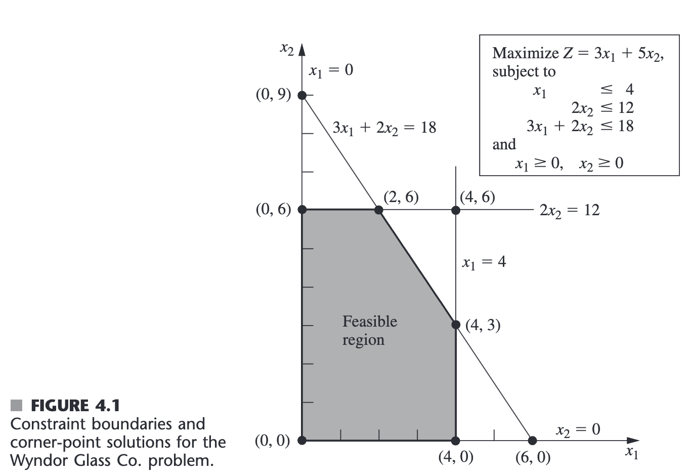
Corresponding terminology for the augmented form: - Augmented solution (拓展解): Solution for the original decision variables augmented by the slack variables - Example: augmenting solution (2,6) yields the augmented solution (2,6,2,0,0) - Basic solution (基本解): Augmented corner-point solution - Example: augmenting corner-point solution (4,6) yields basic solution(4,6,0,0,-6) - Basic feasible (BF) solution (基本可行解): Augmented CPF solution - Example: the CPF (0,6) is equivalent to the BF solution (0,6,4,0,6)
Note: CPF (and BF) solution can be either feasible feasible or infeasible. 基本可行解(BF solution)是拓展的 CPF 解。
The only difference between basic solutions and corner-point solutions (or betweenBF solutions and CPF solutions) is whether the values of the slack variables are included
This fact gives us 2 degrees of freedom in solving the system, since any two variables can bechosen to be set equal to any arbitrary value in order to solve the three equations in terms ofthe remaining three variables
A basic solution has the following properties: 方程结构: 基变量个数=约束条件数 非基变量个数(自由度) = 变量总数-约束条件数
一个基本解具有如下性质: 1. 每个变量都可以作为非基变量或基变量 2. 基变量的个数等于约束条件数。因此 非基变量数 = 变量总数减去约束条件个数 3. 非基变量的值设为 0 4. 基变量的值作为方程组的联立解被求得。 5. 如果基变量满足非负约束,基本解为 BF 解
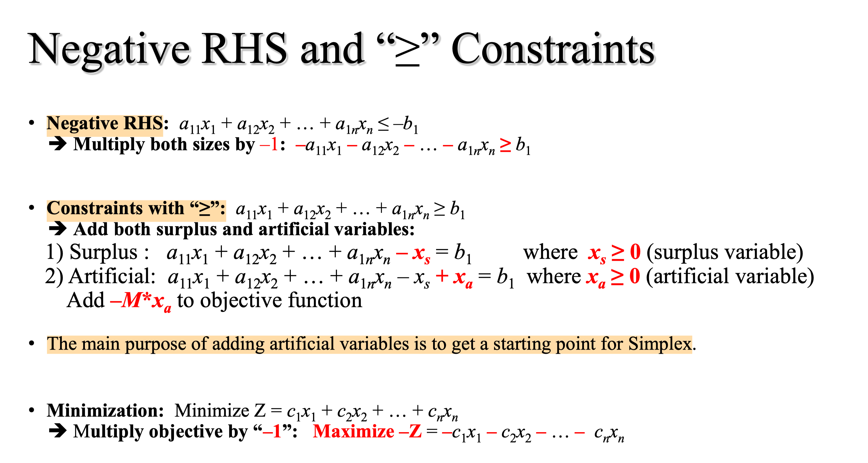
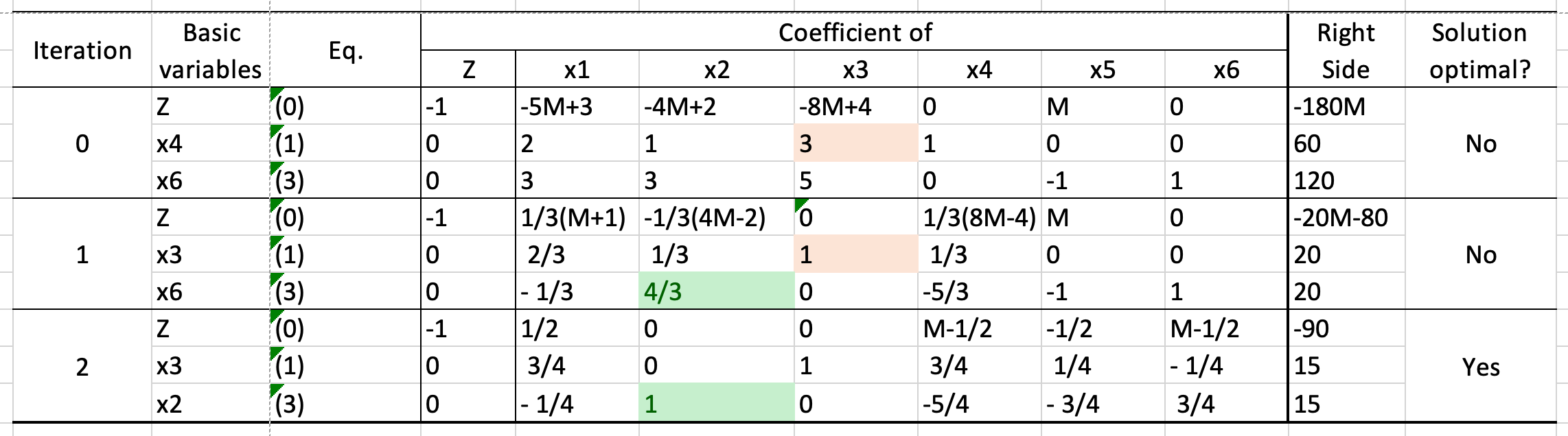
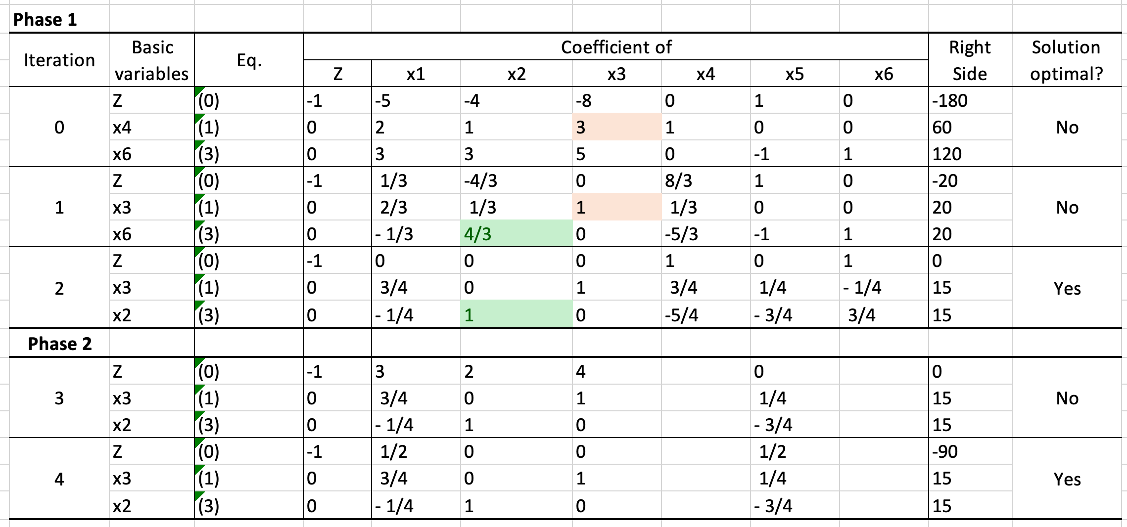
求解等号或大于约束: - Big M method
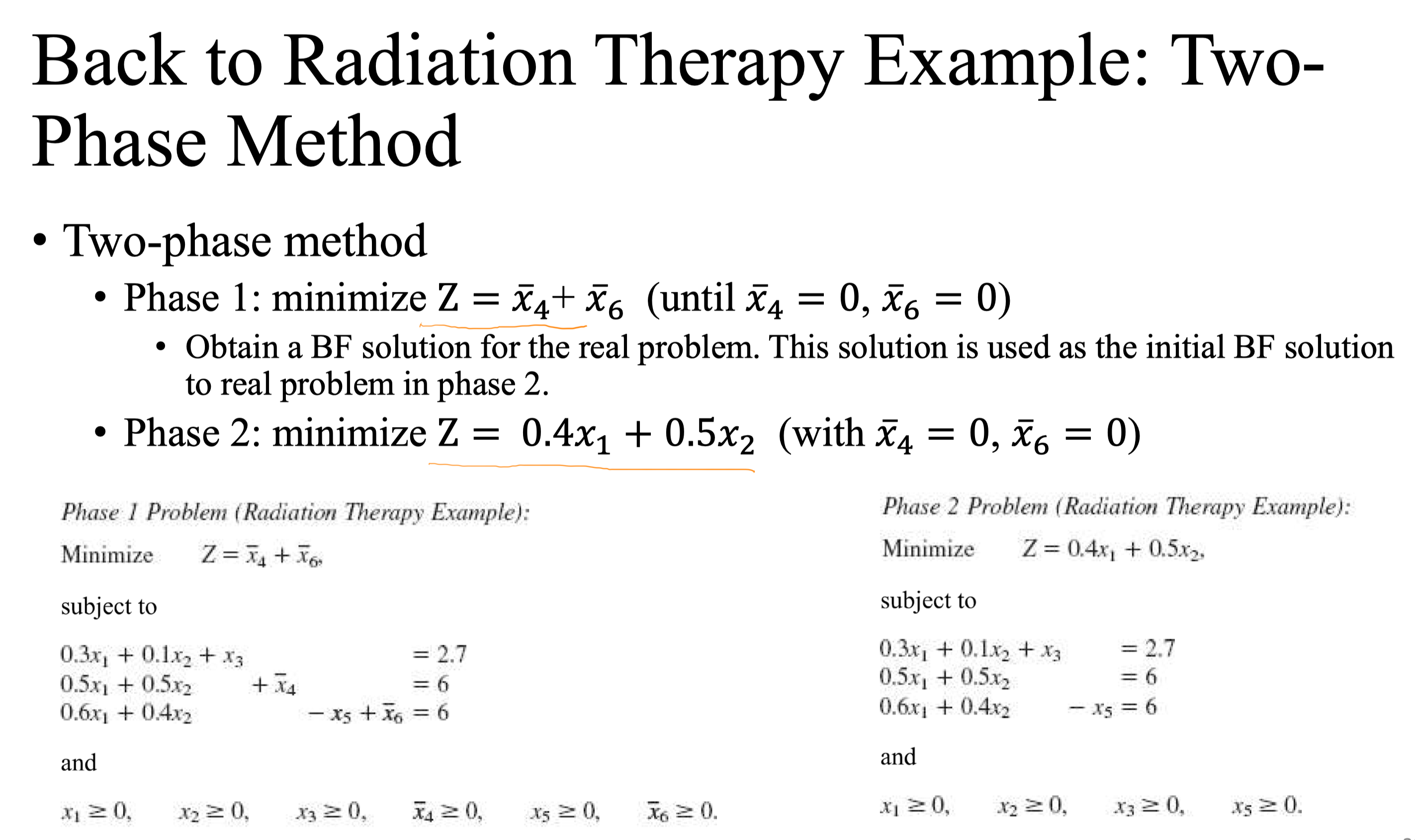
- Two phase method
5. Theory of the Simple Method
5.1 Foundations of the Simplex Method
A corner-point feasible (CPF) solution is a feasible solution that does not lieon any line segment1 connecting two other feasible solutio
Properties of CPF Solutions CPF 解的性质 1. 1)如果只有一个是最优解,他一定是 CPF 解;2)如果有许多最优解(在有界可行域重),至少两个必为相邻 CPF 解 2. 只有有限个 CPF 解 3. 如果一个 CPF 解没有相邻 CPF 解比它更优(以 Z 来衡量),那么就不存在任何更好的 CPF 解。这样,假定这个问题至少有一个最优解(由问题具有可行解和一个有界的可行鱼来保证),这个 CPF 解就是最优解(性质一)。
5.2 The Simplex Method in Matrix Form
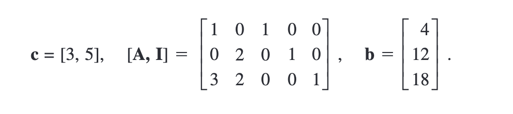
Using matrices, the standard form can be given by: \max Z = cX subjective to Ax \le b \quad \text{and} \quad x \ge 0,
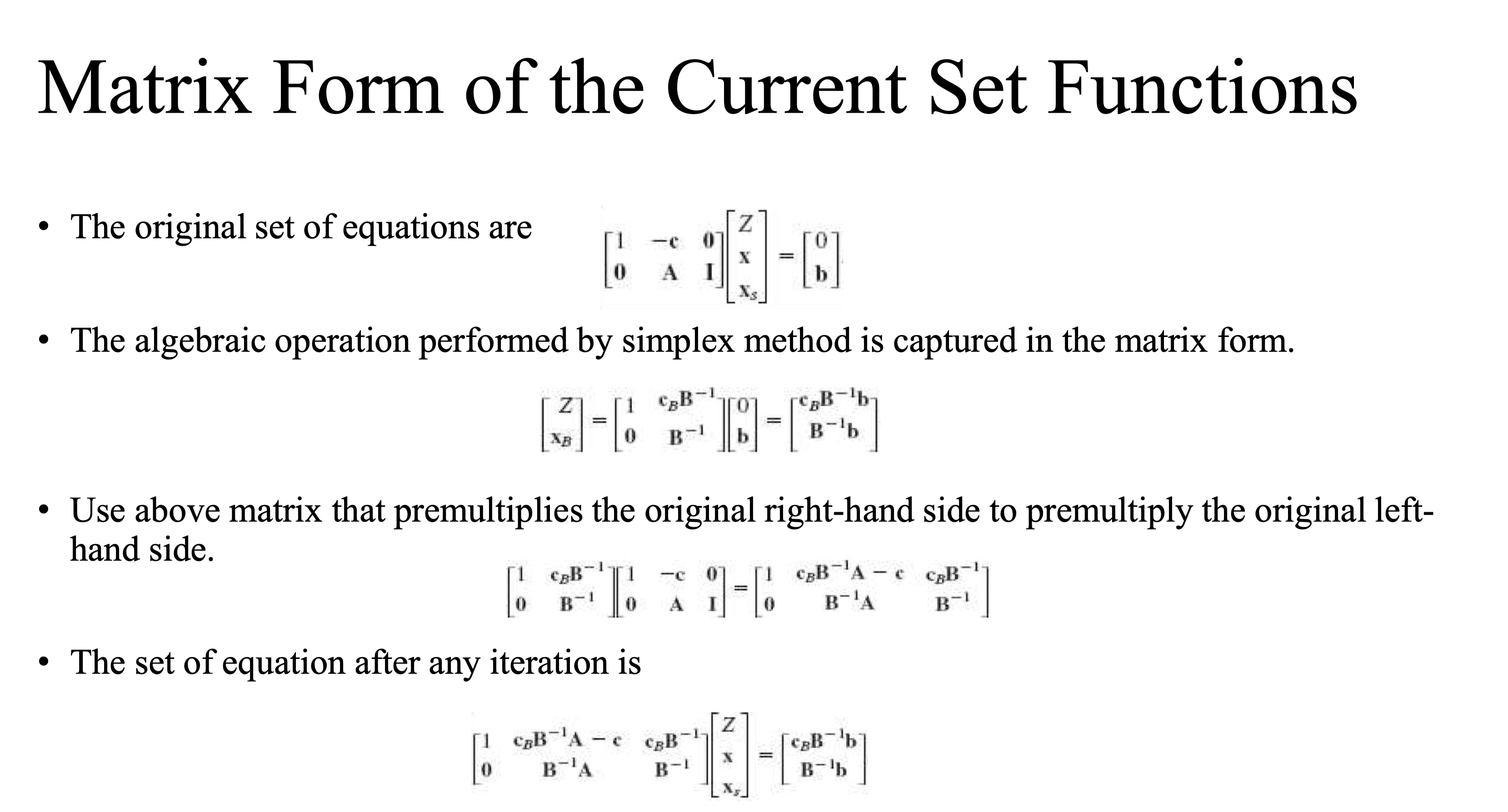
Summary of the Matrix form of the simples solution - Initialization: Introduce slack variable to obtain initial basic variable. This yields initial 𝑥 𝐵 , 𝑐 𝐵 ,𝐵 . - Iteration Step 1: Determine the entering basic variable - Check coefficient of nonbasic variable in Eq(0) - Select negative coefficient having the largest value Step 2. Determine the leaving basic variable - Use B^{-1}A , x_B = B^{-1} b and minimal ratio Step 3. Determine the new BF solution - Update 𝐵, 𝑥_𝐵 , 𝑐_𝐵 Optimality test: The solution is optimal iff positive c_B B^{-1} A - c and c_B B^{-1} are positive.
E.g. 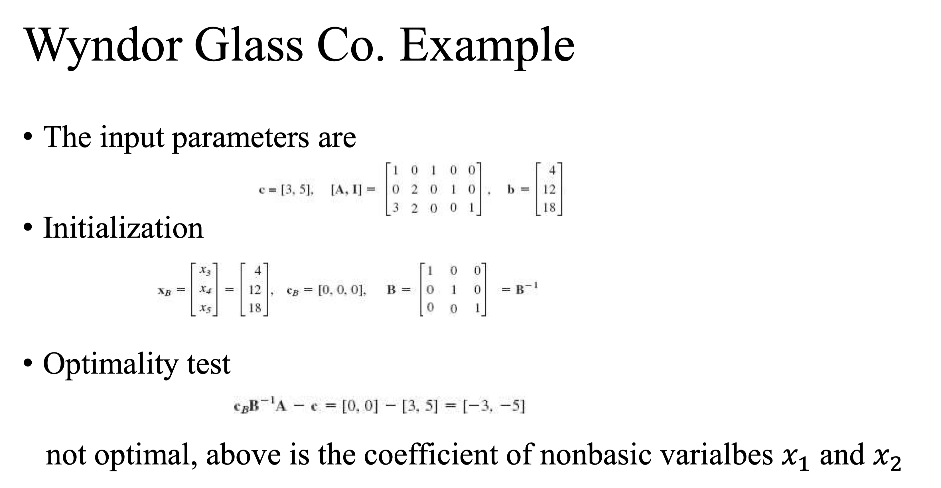
These appli-cations are particularly important only when we are dealing with the final simplex tableauafter the optimal solution has been obtained
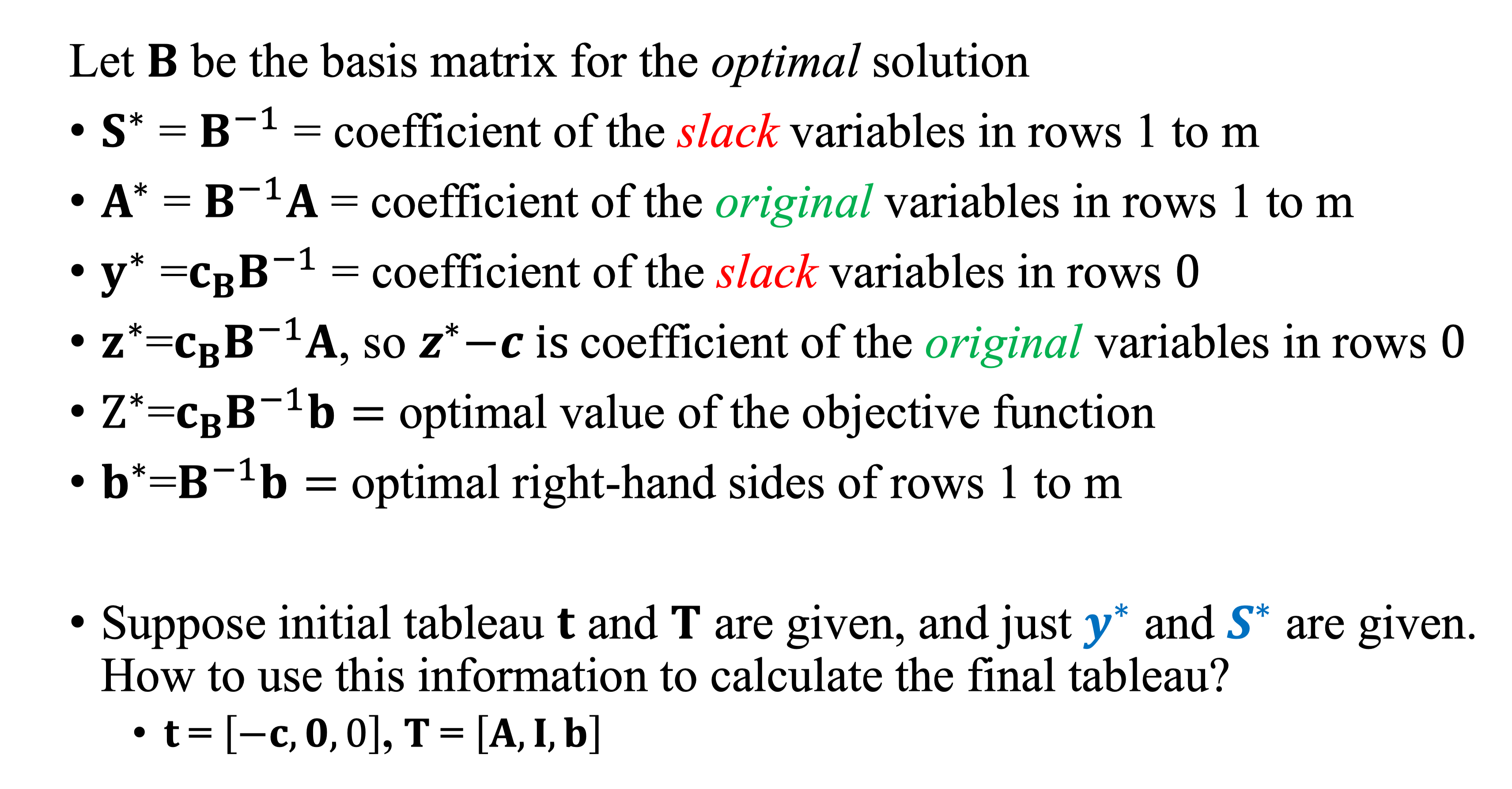
设 B 是用单纯形法找出最优解时的基矩阵,令 - S^*=B^{-1} 表示第一行至 m 行中 松弛变量 的系数 - A^*=B^{-1}A 表示第一行至 m 行中 原变量 的系数 - y^*=c_B B^{-1} 表示第 0 行中 松弛变量 的系数 - z^*=c_B B^{-1} A ,所以 z^* - c=0 为第 0 行中原变量的系数 - Z^*=c_B B^{-1} b 表示目标函数的最优值 - b^*=B^{-1} b 表示第一行至 m 行最优的右端项值
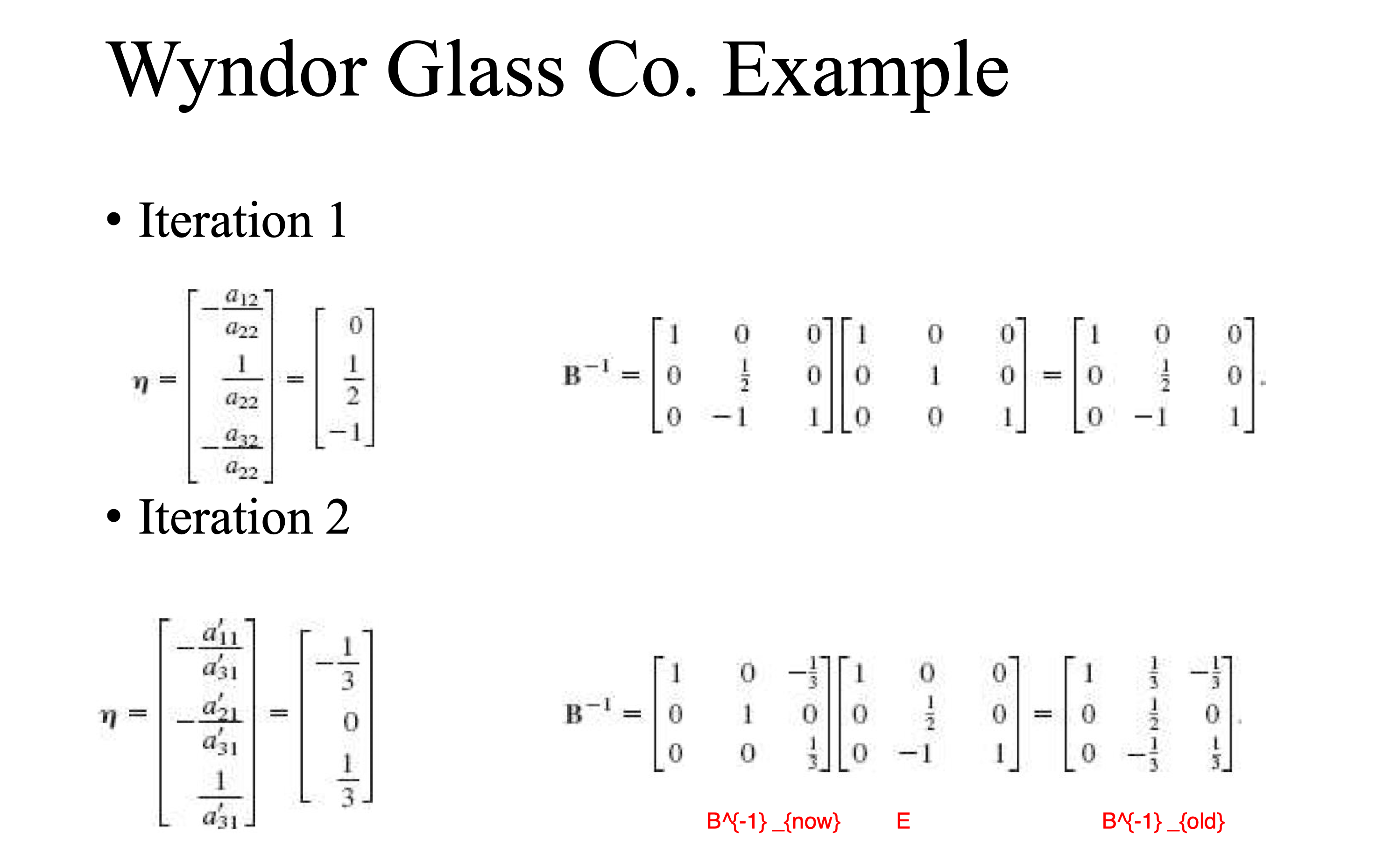
5.4 The Revised Simplex Method
\left(\mathbf{B}_{\text {new }}^{-1}\right)_{i j}=\left\{\begin{array}{ll} \left(\mathbf{B}_{\text {old }}^{-1}\right)_{i j}-\frac{a_{i k}^{\prime}}{a_{r k}^{\prime}}\left(\mathbf{B}_{\text {old }}^{-1}\right)_{r j} & \text { if } i \neq r \\ \frac{1}{a_{r k}^{\prime}}\left(\mathbf{B}_{\text {old }}^{-1}\right)_{r j} & \text { if } i=r . \end{array}\right.
6. Duality theory
This discovery re-vealed that every linear programming problem has associated with it another linear pro-gramming problem called the dual.
The relationships between the dual problem and theoriginal problem (called the primal) prove to be extremely useful in a variety of ways
6.1 The Essence of Duality Theory
Given our standard form for the primal problem at the left (perhaps
after conversion fromanother form), its dual problem has the form shown
to the right. 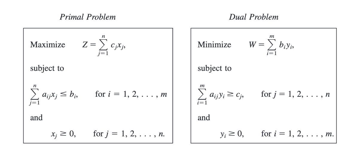
原问题可以理解为最大利润,对偶问题为最小化成本,所以的得到影子价格,构成目标函数的参数。
Summary of Primal-Dual Relationships Summary of Primal-Dual
Relationships 1. Weak duality property: If x is a feasible solution for the
primal problem and y is a feasible solution for the dual problem, then
cx ≤ yb. One application of the dual is
to provide a bound for the optimal value. 2. Strong duality
property: If x^* is an
optimal solution for the primal problem and y* is an optimal
solution for the dual problem, then cx^* =
y^*b.
这说明,当两个问题中有一个不是最优解,或者两个都不是最优解时,会有 cx<yb.
且当两个都是最优解的时候(目标函数相等),则是 cx=yb 3. Complementary solutions
property: At each iteration, it simultaneously identifies a
CPF solution x for the primal
problem and a complementary solution (互补解) y for the dual problem, and cx=yb 4. Complementary optimal
solutions property: At the final iteration, it simultaneously
identifies a optimal solution x^* for the primal problem and a
complementary optimal solution (最优互补解) y for the dual problem, and cx^*=y^* b 5. Symmetry
property:
对于任意一个远问题和他的对偶问题,两个问题之间的一切关系必定是对称的。
6. Duality Property: The following are the only
possible relationships between the primal and dual problems.
-
如果一个问题拥有可行解和有边界的目标函数(存在最优解),那么另一个问题也会有可行解和有界的目标函数。If
one problem has feasible solutions and a bounded objective function (and
so has an optimal solution), then so does the other problem, so both the
weak and strong duality properties are applicable.
- 如果一个问题拥有可行解,
但是目标函数是无界的(无最优解),那么另一个问题没有可行解。If one
problem has feasible solutions and an unbounded objective function (and
so no optimal solution), then the other problem has no feasible
solutions. -
如果一个问题没有可行解,那么另一个问题或者没有可行解,或者有可行解,但是目标函数无界。If
one problem has no feasible solutions, then the other problem has either
no feasible solutions or an unbounded objective function
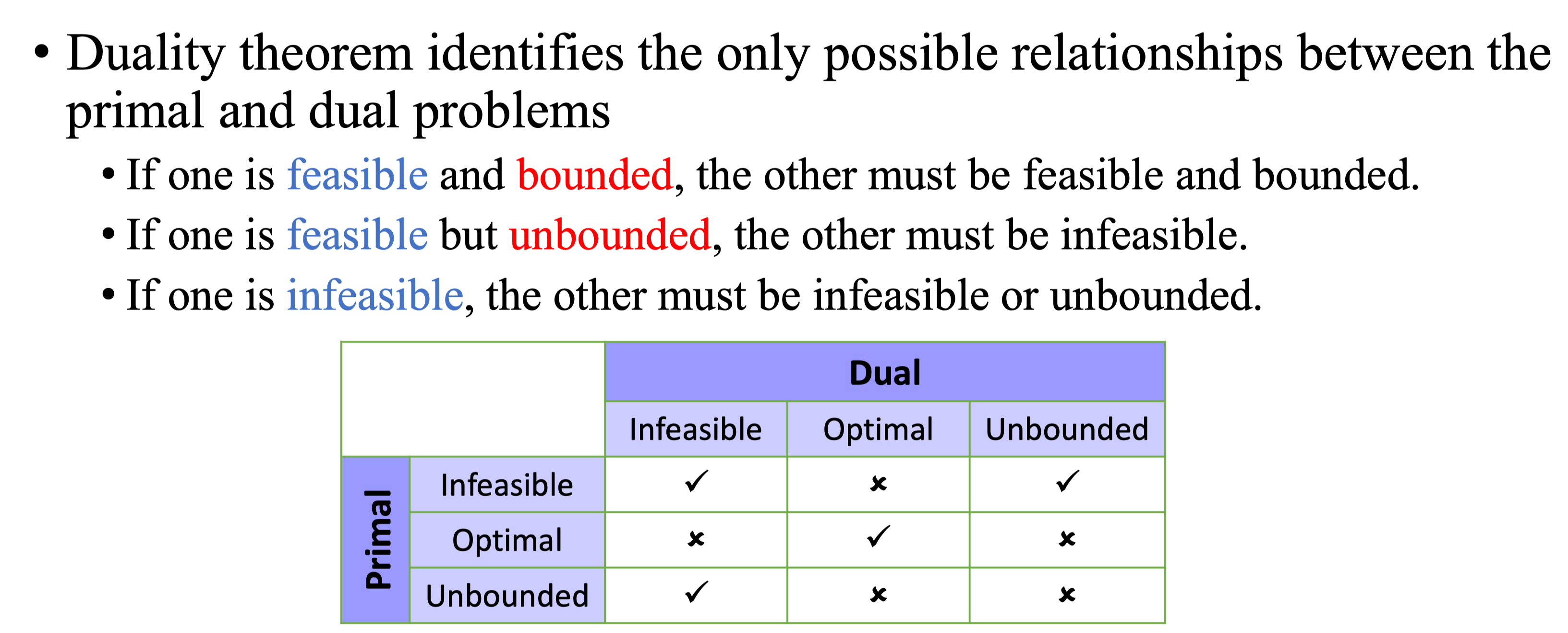 Note: Feasible refers to
feasible zone, bounded refers to objective function
Note: Feasible refers to
feasible zone, bounded refers to objective function
6.3 Prime-Dual Relationship
Complementary slackness property
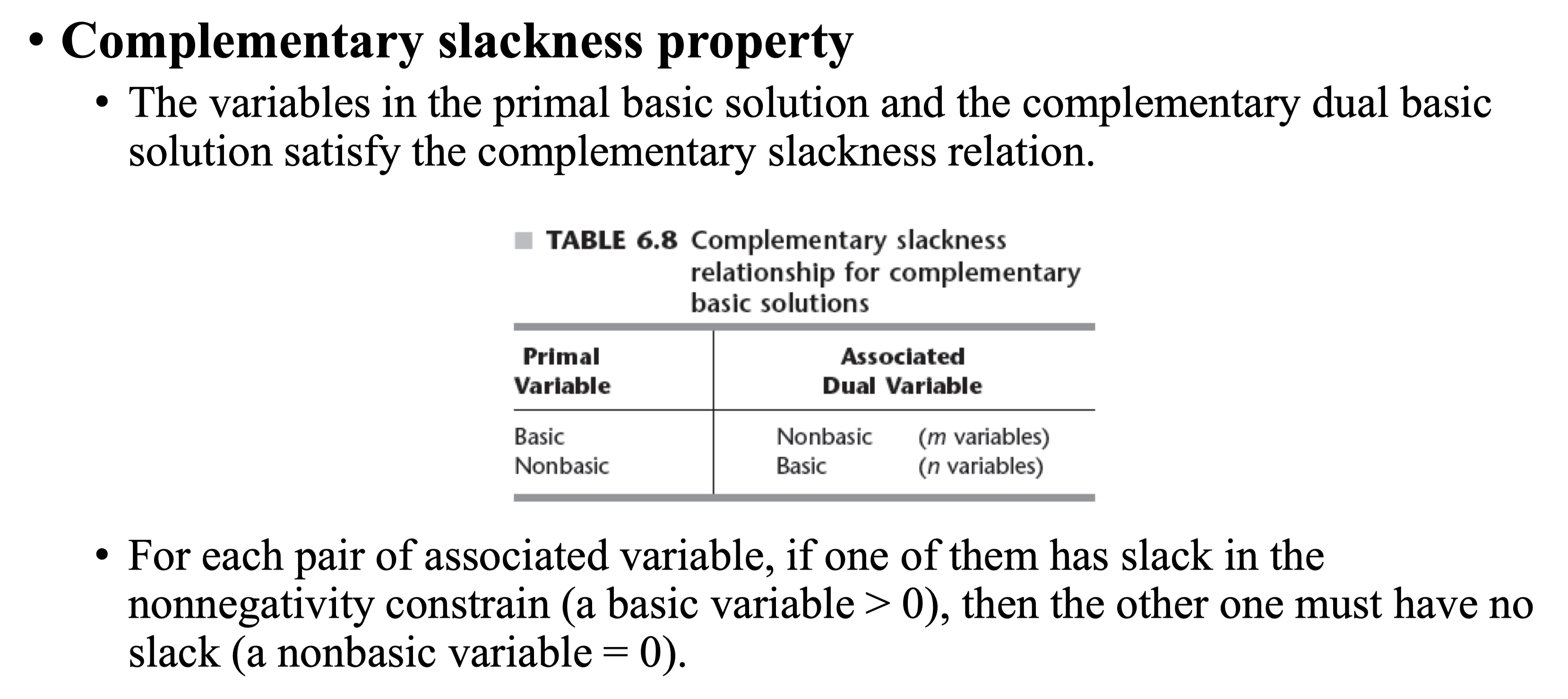
Complementary slackness property: Given the association between variablesin Table 6.7, the variables in the primal basic solution and the complementarydual basic solution satisfy the complementary slackness relationship shown inTable 6.8. Furthermore, this relationship is a symmetric one, so that these twobasic solutions are complementary to each other.
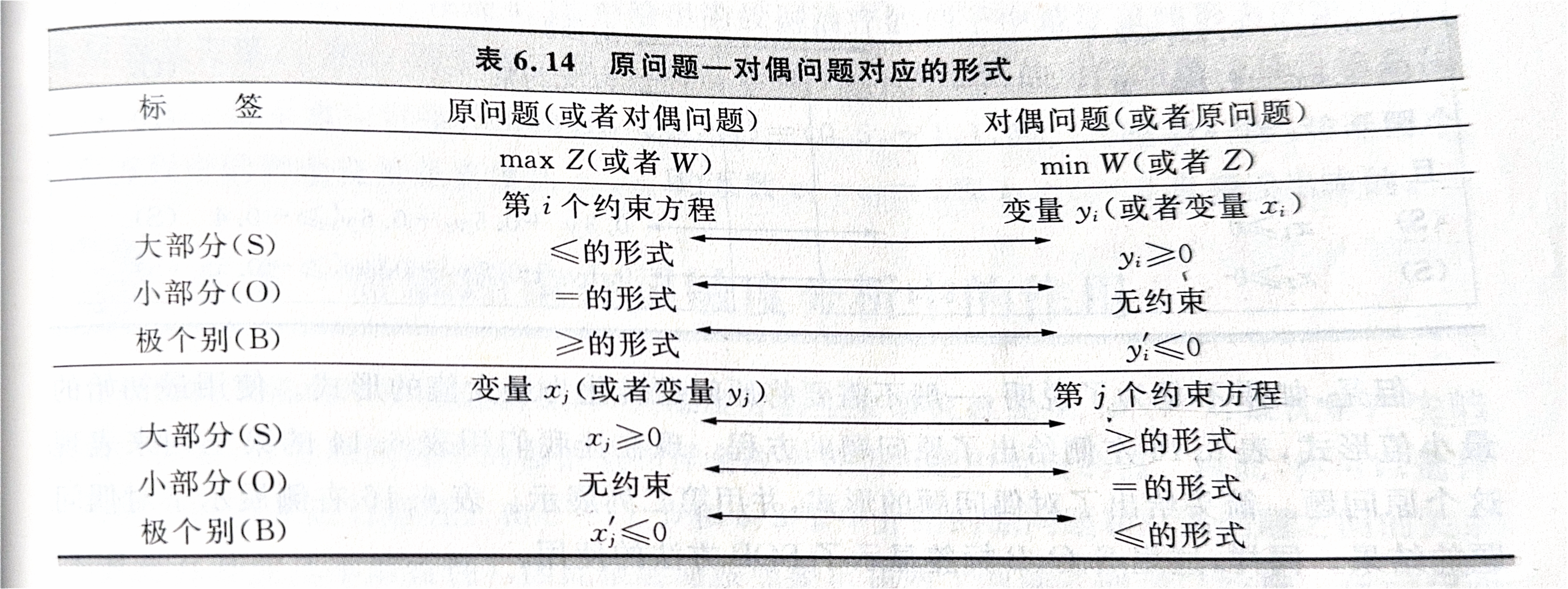
6.4 Adapting to Other Primal Forms
- Sensible-odd-bizarre (大部分、小部分、极个别方法)
The sensible-odd-bizarre method, or SOB method for short, saysthat
the form of a functional constraint or the constraint on a variable in
the dual problemshould be sensible, odd, or bizarre 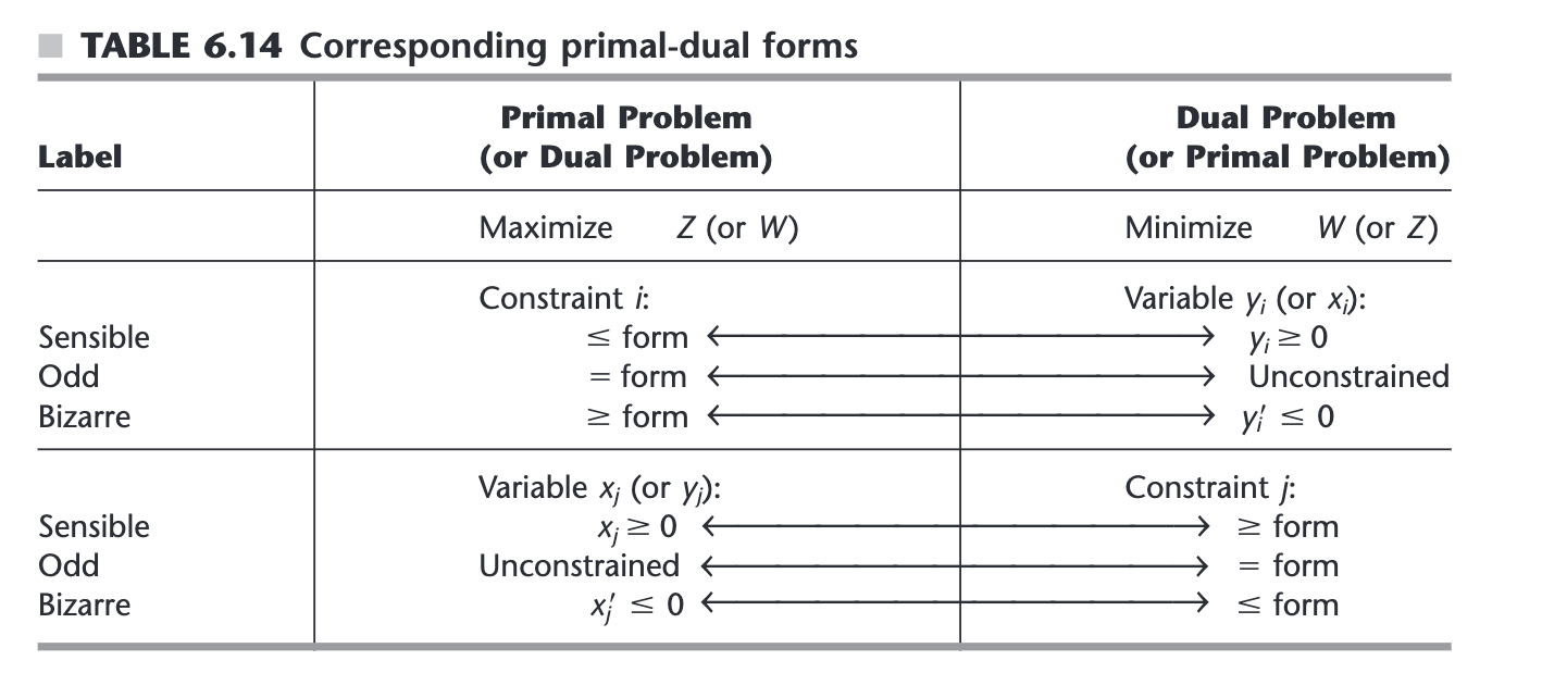
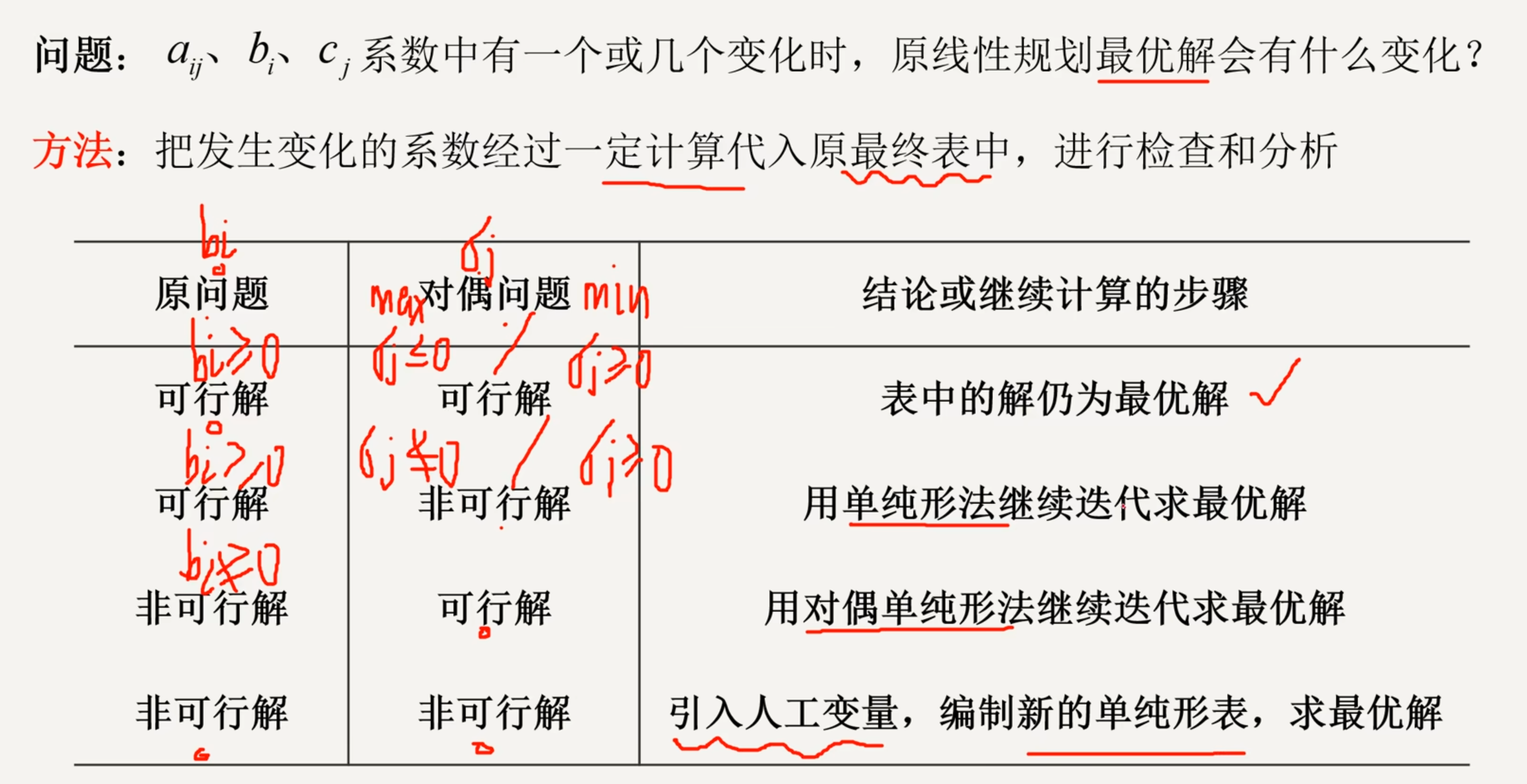
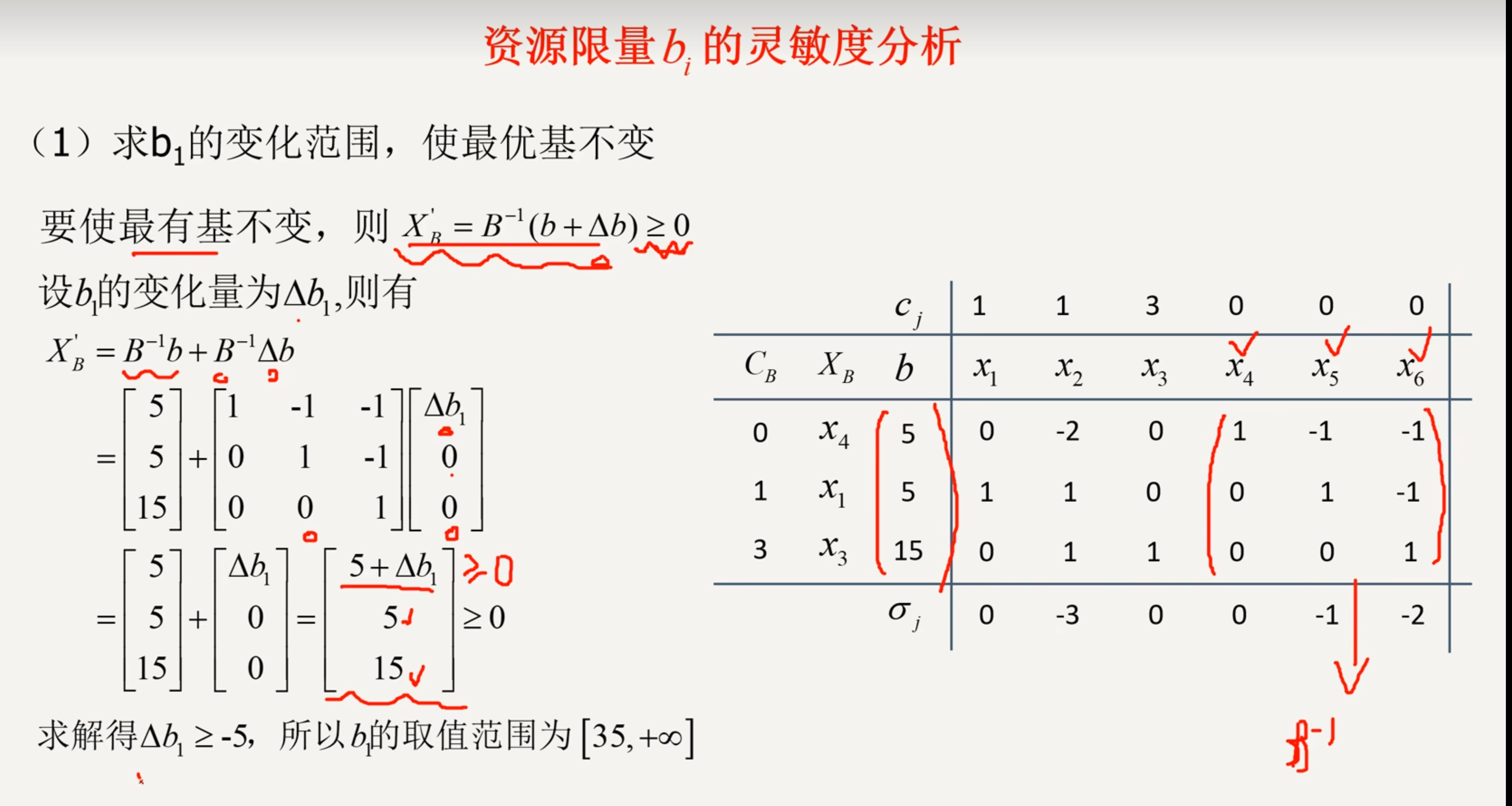
6.7 Sensitive Analysis
13 nonlinear Programming
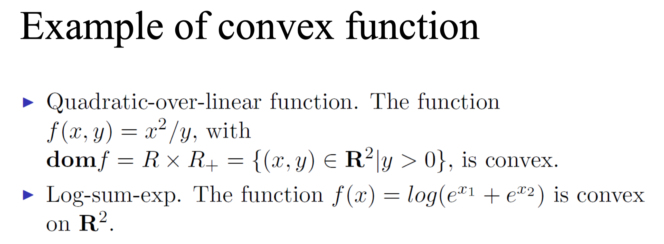
Types of Nonliear Programming Problems - Unconstrained optimization - Minimize f(x) for all values of x = (x_1 , x_2, \cdots, x_n ) - No constraints - Linearly constrained optimization - All constraint functions are linear - Objective function is nonlinear - Quadratic programming - Linear constraints - Objective function is quadratic and convex - Separable programming Each term involves just a single variable The function is separable into a sum of functions of individual variables f(x) = \sum\limits_{j=1}^n f_j (x_j) - Nonconvex programming Functions do not satisfy assumptions of convex programming No algorithm will find an optimal solution for all such problems Some algorithms explore various parts of the feasible region and may find a global maximum - Convex programming f(x) and g_i(x) are convex functions - Geometric programming - Fractional programming
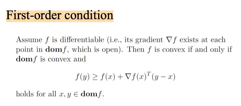
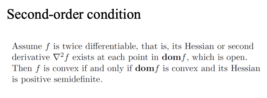
convex function: A function f: R^n \to R is convex if dom f is a convex set and if for all x, y \in dom f and \theta with 0\leq \theta\le 1, we have: f(\theta x + (1-\theta)y \le \theta f(x) + (1-\theta)f(y)
函数为凹函数,则二阶导数大于0;函数为凸函数,则二阶导数小于零.
Operation that preserve convexity 
 - Nonnegative weighted
sums
f = w_1 f_1 + \cdots + w_m f_m
- Pointwise maximum and supremum If f_1 and f_2
are convex functions then their pointwise maximum f, defined by f(x)
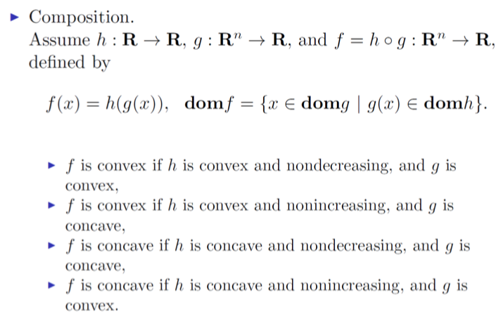
= \max \{f_1(x),f_2(x)\}, is also convex - Composition
- Nonnegative weighted
sums
f = w_1 f_1 + \cdots + w_m f_m
- Pointwise maximum and supremum If f_1 and f_2
are convex functions then their pointwise maximum f, defined by f(x)
= \max \{f_1(x),f_2(x)\}, is also convex - Composition
CONVEX OR CONCAVE FUNCTIONS OF SEVERAL VARIABLES KKT condition 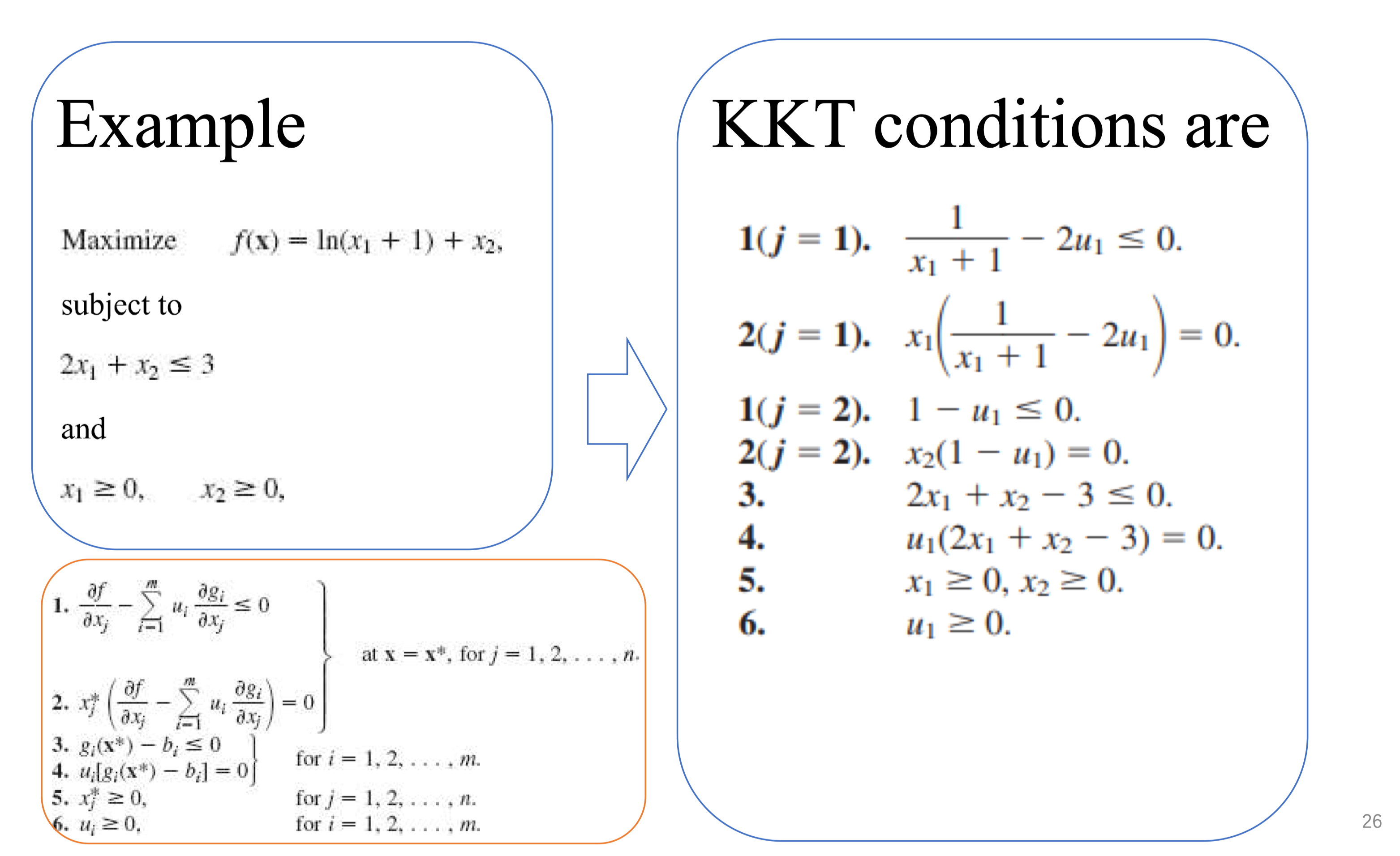
E.g. Ex. 5 Consider the following convex programming problem: \begin{align*} \quad \text{Maximize} \qquad f(x) = 24 x_1- x_1^2 + 10 x_2 - x_2^2 \end{align*} subject to \begin{align*} x_1 \leq 10\\ x_2 \leq 15 \end{align*} and x_1 \geq 0, \quad x_2 \geq 0
- Use the KKT conditions for this problem to derive an optimal solution.
Solution for 5a
Let \begin{align*} F(x) &= f(x) -\alpha g(x_1) - \beta g(x_2)\\ &=24 x_1 - x_1^2 + 10 x_2 -x_2^2 -\alpha(x_1 -10) -\beta(x_2-15) \end{align*} where \alpha, \beta >\geq 0. According to the KKT theorem, for the problem, we can get the following conditions: \begin{align*} \frac{\partial F(x)}{\partial x_1} = 24 - 2x_1 - \alpha \leq 0 \\ \frac{\partial F(x)}{\partial x_2} = 10 - 2x_2 - \beta \leq 0 \\ x_1 \frac{\partial F(x)}{\partial x_1} = x_1(24 - 2x_1 - \alpha) = 0 \\ x_2 \frac{\partial F(x)}{\partial x_2} = x_2 (10 - 2x_2 - \beta) = 0 \\ \alpha (x_1 - 10) = 0\\ \beta (x_2 - 15) = 0 \\ x_1 - 10 \leq 0\\ x_2 - 15 \leq 0 \\ x_1, x_2, \alpha, \beta \geq 0 \end{align*} Then, we can solve the above system, get the following result: \begin{align*} x_1 = 10 \\ x_2 = 5\\ \alpha = 4\\ \beta = 0 \end{align*} Thus, the optimal maximum results is f(x) = 24\times 10 - 10^2 + 10\times 5 - 5^2 = 165