1. Introduction

Blending 集成方法的学习过程中，可以发现 Blending 在集成过程中只使用到了验证集的数据，这就造成了很大的浪费。因此可以靠用使用 Stacking 集成方法进行改进。

Blending 产生验证集的方式是使用分割的方式，产生一组训练集和验证集，那么是否可以将这种方式改进为交叉验证的方式呢？于是就有了如下的 Stacking 集成方法，其步骤如下：

记初始训练集为 Train set，测试集为 Test set，shape 分别为 (train_size, 1) 和 (test_size, 1)。将 Train set 划分为多个部分（如 10 个），如下图 (Source: Analytics Vidhya)；

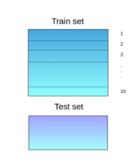
用划分后的的 9/10 作为训练集 (train_set) 训练基准模型 (如决策树)，并用训练好的模型对剩下的 1/10 数据 (验证集, val_set) 和测试集 (Test_set) 来预测数据；
重复迭代训练 10 次直到所有数据都作为 val_set，并将 val_set 的 10 份预测的数据拼接为一个 shape 为 (train_size, 1) 的矩阵 (记为 Trainset)。
对迭代过程中得到的 10 份测试集 (Test set) 的预测数据取加权平均，得到一个shape 为 (test_size, 1)的矩阵。
重复步骤 2-4 训练其他基准模型 (如 knn) :
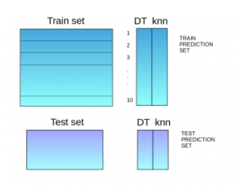
将上述训练得到的一系列 Trainset 串联，得到一个形状为 (train_size, num_features) 的矩阵，并用该矩阵训练第二层的模型，然后用训练好的新模型来做测试集的预测，并作为最终预测结果。

下面借助实例来体验 Stacking 的魅力（参考案例：cnblogs）：注：sklearn 模块并没有 Stacking 的方法，因此需要使用 mlxtend 工具包。

2. A example of stacking model

2.1 Data process

Import modules

import numpy as np
import pandas as pd
import matplotlib.pyplot as plt

from sklearn.model_selection import cross_val_score
from sklearn.linear_model import LogisticRegression
from sklearn.neighbors import KNeighborsClassifier
from sklearn.naive_bayes import GaussianNB
from sklearn.ensemble import RandomForestClassifier
from mlxtend.classifier import StackingCVClassifier

from sklearn.metrics import accuracy_score as ac
from sklearn.model_selection import train_test_split
%matplotlib inline

Load data 本案例使用了 Kaggle 比赛中的一份泰坦尼克号乘客的数据来进行处理，下载链接：Titanic-data.csv
1
data = pd.read_csv('./titanic-data.csv')
Information:
- PassengerId：乘客ID
- Survived：是否获救，用1和Rescued表示获救,用0或者not saved表示没有获救
- Pclass：乘客等级，“1”表示Upper，“2”表示Middle，“3”表示Lower
- Name：乘客姓名
- Sex：性别
- Age：年龄
- SibSp：乘客在船上的配偶数量或兄弟姐妹数量）
- Parch：乘客在船上的父母或子女数量
- Ticket：船票信息
- Fare：票价
- Cabin：是否住在独立的房间，“1”表示是，“0”为否
- embarked：表示乘客上船的码头距离泰坦尼克出发码头的距离，数值越大表示距离越远

Statistical description

1	data.info() # See datatype

Results:

<class 'pandas.core.frame.DataFrame'>
RangeIndex: 891 entries, 0 to 890
Data columns (total 12 columns):
 #   Column       Non-Null Count  Dtype  
---  ------       --------------  -----  
 0   PassengerId  891 non-null    int64  
 1   Survived     891 non-null    int64  
 2   Pclass       891 non-null    int64  
 3   Name         891 non-null    object
 4   Sex          891 non-null    object
 5   Age          714 non-null    float64
 6   SibSp        891 non-null    int64  
 7   Parch        891 non-null    int64  
 8   Ticket       891 non-null    object
 9   Fare         891 non-null    float64
 10  Cabin        204 non-null    object
 11  Embarked     889 non-null    object
dtypes: float64(2), int64(5), object(5)
memory usage: 83.7+ KB

Missing values processing
- Embarked
  
  Embarked 列仅有两个缺失值，而 'S' 占比最高，故将缺失值用 'S' 填充；
  1
  data['Embarked'] = data['Embarked'].fillna('S')
- Age
  
  Age 包含较多缺失值，用均值填充；
  1
  2
  dmean_age = data['Age'].mean()
  data['Age'] = data['Age'].fillna(mean_age)
- Cabin
  
  Cabin 值缺失过多，且每位乘客房间号均不一样，且无规律，故舍去。

Datatype transformation

Sex 将性别转换未数值型数据，用 0 表示男性，1 表示女性

1 2	data.loc[data['Sex'] == 'male', 'Sex'] = 0 # 'male' -> 0 data.loc[data['Sex'] == 'female', 'Sex'] = 1 # 'female' -> 1

Embarked

将 'C' 所在位置的值改为 1, 'S' 所在位置的值改为 2, 'Q' 所在位置的值改为 3；

1
2
3

data.loc[data['Embarked'] == 'C', 'Embarked'] = 1 # 'C' -> 1
data.loc[data['Embarked'] == 'S', 'Embarked'] = 2 # 'S' -> 2
data.loc[data['Embarked'] == 'Q', 'Embarked'] = 3 # 'Q' -> 3

Drop irrelevant variables

1
2
3

columns = data.columns
columns = columns.drop(['PassengerId', 'Cabin', 'Name', 'Ticket'])
data = data.loc[:, columns]

Parameters setting 可以直到 data的列名称为 ['Survived', 'Pclass', 'Sex', 'Age', 'SibSp', 'Parch', 'Fare', 'Embarked']。选择最后一列作为分类标准。

test_percent = 0.10 # 测试集大小

train_X = train.loc[:, data.columns[1:]]
train_Y = train.loc[:, data.columns[0]].values.reshape(-1,)
test_X = test.loc[:, data.columns[1:]]
test_Y = test.loc[:, data.columns[0]].values.reshape(-1,)

2.2 Creating Stacking model

Stacking

RANDOM_SEED = 42

# The first layer
clf1 = KNeighborsClassifier(n_neighbors=1)
clf2 = RandomForestClassifier(random_state=RANDOM_SEED)
clf3 = GaussianNB()
lr = LogisticRegression()

# Starting from v0.16.0, StackingCVRegressor supports
# `random_state` to get deterministic result.
sclf = StackingCVClassifier(
      classifiers=[clf1, clf2, clf3],  # The first layer
      meta_classifier=lr,   # THe second layer
      random_state=RANDOM_SEED)

print('3-fold cross validation:\n')

for clf, label in zip([clf1, clf2, clf3, sclf], ['KNN', 'Random Forest', 'Naive Bayes','StackingClassifier']):
    scores = cross_val_score(clf, train_X, train_Y,
              cv=3, scoring='accuracy')
    print("Accuracy: %0.2f (+/- %0.2f) [%s]" % (scores.mean(),
               scores.std(), label))

Result:

3-fold cross validation:

Accuracy: 0.70 (+/- 0.02) [KNN]
Accuracy: 0.80 (+/- 0.01) [Random Forest]
Accuracy: 0.76 (+/- 0.02) [Naive Bayes]
Accuracy: 0.79 (+/- 0.01) [StackingClassifier]

Ploting decision region 由于使用了多维数据，决策边界暂无法成功绘制，有时间了再琢磨。

3. Conclusion

3.1 Blending 和 Stacking 对比

Blending 优点：
- 比 Stacking 简单，不用进行 K 次的交叉验证来获得 stacker feature
缺点：
- 在训练第二层的模型的时候，仅使用了很少的数据；
- 由于第二层训练数据较少，容易导致过拟合
- stacking 使用多测的 CV 会比较文件。

独孤诗人的学习驿站

Ensemble-Stacking