1 Stata operation
1.1 Import data
use
grilic_small.dta文件的目录请根据自己的文件目录填写,数据文件可在陈强老师的网站下载,Click here,选择《计量经济学及Stata应用》中的数据集下载。1
use "D:\Demo\University\XMU\Class_files\Econometrics\Econometrics and Stata application\Data-Finished-bachelor\grilic_small.dta", clear
clear
关闭一个数据集,以便使用另外一个数据集
describe1
2# 查看数据集中的变量名称、标签等
describe or dset more off/on
1
2
3
4
5# 连续滚屏显示命令运行结果
set more off
# 分页显示命令运行结果
set more onlist1
2
3
4
5
6
7
8
9
10# 查看变量 s 和 lnw 的前 5 个数据
list s lnw in 1/5 # or
l s lnw in 1/5
# 罗列第 11-15 个观测值
list ss lnw in 11/15
# 列出满足条件 ‘s>=16' 的数据
list s lnw if s >= 16
# >=: 等于 <=:小于等于 ==:等于 ~= or !=:不等于 =:赋值drop / keep
1
2
3
4
5
# 删除满足 ’s>=16' 的观测值
drop if s >= 16
# 只保留满足 's>=16' 的观测值
keep if s >= 16注:Stata 并不提供 undo 功能,故需慎重删除数据,最好保留备份-
sort / gsort
1
2
3
4
5
6
7# 将数据按照变量 s 的升序排列
sort s
lsit
# 降序排列
gsort -s
list
1.2 Plot
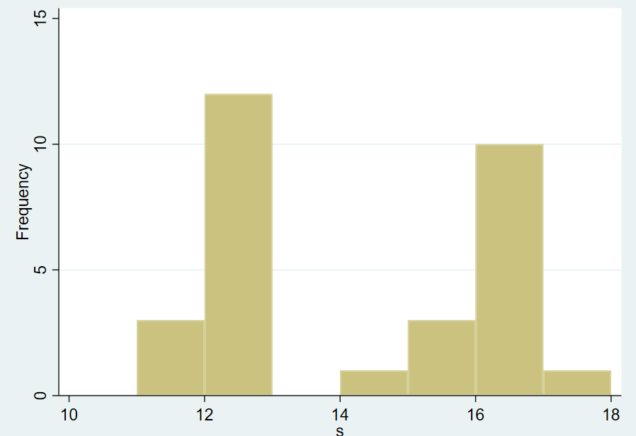
1.3.1 直方图
1 | histogram s, width(1) frequency |
Result:
- 查看帮助文档
对于任何 Stata 命令,只需要输入
help command_name
即可查看该命令的帮助文档,初学者应养成经常查看帮助文档的习惯。
1 | help histogram |
Result:
1 | histogram varname [if] [in] [weight] [, [continuous_opts | discrete_opts] options] |
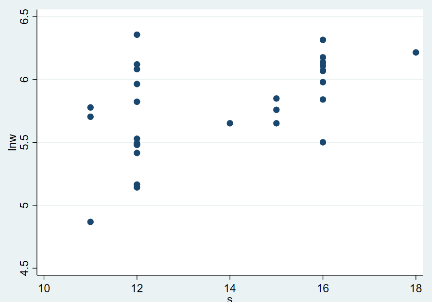
1.3.2 散点图
1 | scatter lnw s |
Result:
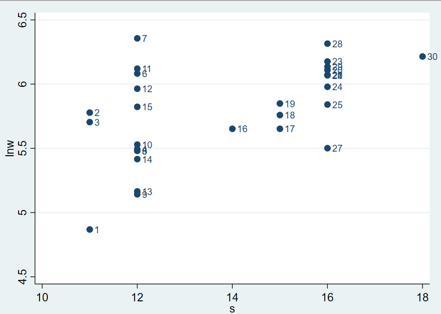
- 标签
如果想在散点图上标注每个点对应于哪个观测值,可先定义变量 n,表示第 n 个观测值:
1 | gen n = _n |
其中,_n 表示第 n
个观测值。然后以变量作为每个点的标签来画散点图。结果如下:
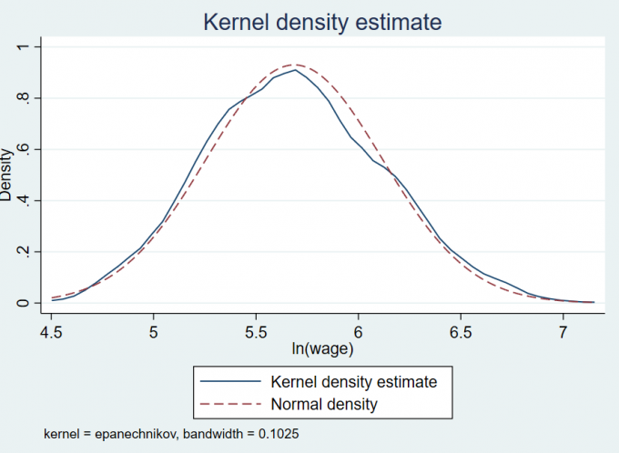
1.3.3 核密度估计图
直方图必然是不连续的,如果想得到密度函数的连续估计,可输入命令:
1 | kdensity lnw, normal normop (lpattern (dash)) |
其中
kdensity:核密度估计(kernel density estimation);normal:画正态分布的密度函数作为对比;normop (lp (Dash)):将正态密度用虚线来画。normop:normal optionslpattern: line pattern.
Result:
1.3 Statistical analysis
统计特征
1
2
3
4summarize s
su s
sum lnw, detail # 显示更多统计指标,如偏度、峰度Result:
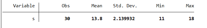
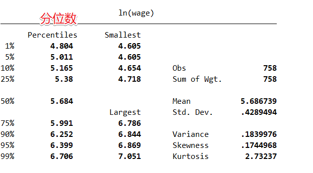
Fig. 1-4 Statistical description
显示了变量 s 的样本容量、平均值、标准差、最小值于最大值。如 不指明变量,则显示 所有变量 的统计指标。
经验累计分布函数(Empirical cumulative distribution function)
1
2tabulate s # 显示 s 的经验累积分布番薯
ta sResult:
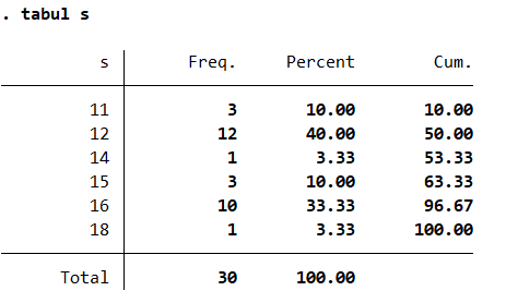
Fig. 1-5 Empirical cummlative distribution
其中,
Freq表示频数,Percent表示百分比,而Cum.表示累积百分比。相关系数
1
2pwcorr lnw s expr, sig star(.05)
# 对工资对数、教育年限于工龄之间的相关系数其中,
pwcorr:pairwise correlation,即两两相关;- 选择项
sig:相关系数的显著性水平,即p-value,列在相关系数的下方 ; - 选择项
star (.05):所有显著性水平小于或等于 5% 的相关系数打赏星号。
Result:
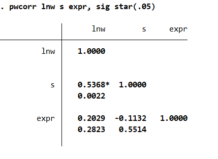
Fig.1-6 Correlation coefficient
结果显示,\rm{ln} w 与 s 的相关系数为 0.5368,且在 1% 水平上显著( p 值为0.0022);\rm{ln} w 与 expr 的相关系数为 -0.1132,但此相关关系也不显著(p-value 为0.5514)
1.4 Generate new variable
1.4.1 Basic operation
- 对数
1 | generate lns = log(s) |
平方
1
gen s2 = s ^2 # 平方项
互动项(乘法)
1
gen exprs = s * expr # s 与 expr 的互动项
指数
1
gen w = exp(lnw) # 指数
1.4.2 虚拟变量
假设定义 s \geq 16 为 ”受过高等教育“,并使用 变量 college 来表示:
1 | gen colleg = (s >= 16) |
其中,括弧 ()
表示对括弧中的表达式进行逻辑评估:如果此表达式为真,则取值为1;如果为假,则取值为0。
变量重命名
1
2rename colleg college
ren colleg college变量重定义
将 ”受过高等教育“的定义改为 s \geq 15,但仍用 college 作为变量名:
1
2
3
4
5
6# Method one
drop college
gen college = (s >= 15)
# Method two
replace college = (s >= 15)变量输入
对于较长的变量,一一输入较为麻烦,,有如下简便方式:
在变量 窗口双击需要的变量;
s1 - s5 来选择这 5 个变量;
用
*来简化变量名的书写。1
drop s* # 去掉所有以 s 开头的变量
1.5 Other
1.5.1 Calculator
Stata 也可作为计算器来使用,命令格式为
display expression。
1 | display log(2) # 计算 ln2 |
1.5.2 Invoke and terminate commands
- 调用旧命令
- 使用键盘上的
Pg Up和Pg Dn键; - 在历史命令窗口 单击 旧命令,将命令调入命令窗口;
- 在历史命令窗口 双击 旧命令,再次执行此命令。
- 使用键盘上的
- 停止执行当前执行命令
- 点击
Break图标的快捷键; - 同时按住
Ctrl + Break。
- 点击
1.5.3 Log file
Stata 日志文件的扩展名为 smcl。可通过快捷键
Log 图标使用,也可通过输入如下命令:
1 | log using today # 在当前路径中生成一个名为 'today.smcl' 的日志文件 |
暂时关闭日志
1
log off
恢复使用日志
1
log on
彻底退出日志
1
log close
1.5.4 Updata stata lib
更新 Stata 命令库(
Stata "ado"文件及其他可执行文件)。
1 | updata all |
非官方命令
最流行的非官方命令下载平台为 统计软件成分 (Statistical Software Components, SSC),从
SCC下载Stata程序的命令为:1
scc install newcommand
如果非官方命令不是来自
SSC,则需要手工安装。只需要将所有相关文件下载到制定的Stata文件夹中即可(通常为ado\plus\)。如果不清楚应把文件复制到哪个文件夹,可输入以下命令,显示Stata的系统路径(System directories):1
sysdir
Result:
1
2
3
4
5
6
7. sysdir
STATA: D:\Program files\Stata 16\
BASE: D:\Program files\Stata 16\ado\base\
SITE: D:\Program files\Stata 16\ado\site\
PLUS: C:\Users\YangSu\ado\plus\ # 复制到此文件夹
PERSONAL: C:\Users\YangSu\ado\personal\
OLDPLACE: c:\ado\
1.5.5 Search and findit
Search command
如果想使用某种估计方法,但不知道它是否存在,可输入命令:
1
search keyword
此命令搜索
Stata帮助文件、Stata常见问题、Stata案例、Stata Journal、Stata Technical Bulletin等。Findit keyword
1
findit keyword
findit搜索范围更广,还包括Stata的网络资源。