1 Series

1.1 Preparation

Import modules
1
2
import pandas as pd
import numpy as np

1.2 Different data type

Time type

1
2
3

>>> t = pd.Timestamp('20180901') # time type
>>> t
Timestamp('2018-09-01 00:00:00')

Created by means of data_range.

>>> dates = pd.date_range('20200101', periods = 6)
>>> dates
DatetimeIndex(['2020-01-01', '2020-01-02', '2020-01-03',
          '2020-01-04','2020-01-05', '2020-01-06'],
           dtype='datetime64[ns]', freq='D')

1.3 Create DataFrame

By dict

# create a dataframe based on dict
df3 = pd.DataFrame({'A':1., 'B':pd.Timestamp('20160901'),
      'C':pd.Series(1,index=list(range(4)),dtype='float32'),
      'D':np.array([3]*4, dtype ='int32'),
      'E':pd.Categorical(['test','train','test','train']),
      'F':'foo'})
print(df3)

Result:

    A       B         C    D     E      F
0  1.0  2016-09-01   1.0   3    test   foo
1  1.0  2016-09-01   1.0   3   train   foo
2  1.0  2016-09-01   1.0   3    test   foo
3  1.0  2016-09-01   1.0   3   train   foo

By Series

1
2
3

# np.nan means NaN
s = pd.Series([1, 3, 5, np.nan, 44, 1])
print(s)

Result:

0     1.0
1     3.0
2     5.0
3     NaN
4    44.0
5     1.0
dtype: float64

By np.array

# create a dataframe based on imported array
df0 = pd.DataFrame(np.random.randn(6,4), index = dates, columns = ['a', 'b', 'c', 'd'])
df1 = pd.DataFrame(np.arange(12).reshape(3,4))
print(df1, df3, sep = '\n')

1.4 Basic information

df3 = pd.DataFrame({'A':1., 'B':pd.Timestamp('20160901'),
      'C':pd.Series(1,index=list(range(4)),dtype='float32'),
      'D':np.array([3]*4, dtype ='int32'),
      'E':pd.Categorical(['test','train','test','train']),
      'F':'foo'})

Dtype of each dimensional
1
df3.dtypes # dimensional type

Row and column index

1 2	df3.index # row index name df3.columns # column name

Statistical description

Describe numerical characteristics, including count, mean, std, min etc.

1	df3.describe() # describe numerical characteristics, including count, mean, std, min etc.

Result:

        A    C    D
count  4.0  4.0  4.0
mean   1.0  1.0  3.0
std    0.0  0.0  0.0
min    1.0  1.0  3.0
25%    1.0  1.0  3.0
50%    1.0  1.0  3.0
75%    1.0  1.0  3.0
max    1.0  1.0  3.0

information

1	df3.info()

Result:

<class 'pandas.core.frame.DataFrame'>
Int64Index: 4 entries, 0 to 3
Data columns (total 6 columns):
 #   Column  Non-Null Count  Dtype         
---  ------  --------------  -----         
 0   A       4 non-null      float64       
 1   B       4 non-null      datetime64[ns]
 2   C       4 non-null      float32       
 3   D       4 non-null      int32         
 4   E       4 non-null      category      
 5   F       4 non-null      object        
dtypes: category(1), datetime64[ns](1), float32(1), float64(1), int32(1), object(1)
memory usage: 288.0+ bytes

1.5 Data type

Specifies the type when creation

import pandas as pd
dfx = pd.DataFrame([['11', 1.2, 3], ['22', 4.8, 5],],
    columns = list('abc'), dtype = np.object)
dfx.dtypes

Result:

a       object
b       object
c       object
dtype:  object

Coercion df.astype()

1 2	dfx[['a', 'b', 'c']] = dfx[['a', 'b', 'c']].astype('float')) dfx.dtypes

Result:

a       float64
b       float64
c       float64
dtype:  object

Turn into numeric pd.to_numeric()

dfy = pd.DataFrame([['11', 1.2, 3], ['22', 4.8, '?'], ],
        columns = list('abc'), dtype = np.object)
dfy['a'] = pd.to_numeric(dfy['a'])
print(dfy.dtypes)

Use pd.apply to apply it to the entire dataframe.

dfy1 = dfy.apply(pd.to_numeric, errors = 'ignore')
 # Igonre and don't change this column when meet errors,
dfy2 = dfy.apply(pd.to_numeric, errors = 'coerce')
 # Transfer the value into NaN when meet errors.
print(dfy.dtypes)
print('-------------------------')
print(dfy2)

Result:

a       int64
b       float64
c       float64
dtype:  object
-------------------------
    a   b    c
0  11  1.2  3.0
1  22  4.8  NaN

2 Choose data

2.1 Basic operation

Import modules and generate datas

import pandas as pd
import numpy as np

df = pd.DataFrame({'A':1., 'B':pd.Timestamp('20160901'),
       'C':pd.Series(1,index=list(arange(4)),dtype='float32'),
       'D':np.array([3]*4, dtype ='int32'),
       'E':pd.Categorical(['test','train','test','train']),
       'F':'foo'})

Row operation

1 2	df2 = df[0:3] # row operation, 0-3 row df2_1 = df[0:1] # single row

Column operation

1 2	df1 = df.A # same sa df.['A'] df2_2 = df['A'] # single column

2.2 Index methods

loc

Select datas by label based index.

1 2	# select by label based index: loc df3 = df.loc[1] # the second row

iloc

Select datas by postitional index.

1 2	# selct by postitional index: iloc df4 = df.iloc[:,1:3] # 1-3 column

ix

Select datas by mixed selection.

1 2	# mixed selection: ix df5 = df.ix[:2,['A', 'D']] # deprecated

2.3 Conditional operation

Logic expression
1
df6 = df[df['A'] > 4]
df['A'] > 4 return the row index which number is bigger than 4, let me name this index as iRow, then df[iRow] return the row date that meets above filter condition.

2.4 Functional methods

tail df.tail(n) returns last n rows from the DataFrame object based on position. It is useful for quickly verifying data. For negative values of n, it returns all rows except the first n rows, equivalent to df[n:].
1
2
3
df.tail() # Default n is 5
df.tail(3) # Return last 3 rows
df.tail(-5) # Return all rows except the first 5 row.

3 DataFrame operation

Preparation

import pandas as pd
import numpy as np

df = pd.DataFrame({'A':1., 'B':pd.Timestamp('20160901'),
    'C':pd.Series(1,index=list(range(4)),dtype='float32'),
    'D':np.array([3]*4, dtype ='int32'),
    'E':pd.Categorical(['test','train','test','train']),
    'F':'foo'})

3.1 Value operation

Set value

Pay attention to the difference.

df.iloc[2, 2] = 111
df.loc[0,'B'] = pd.Timestamp('20180901')
# Note: below command will create a new column named (0, 'B') which values are given
df[0,'B'] = pd.Timestamp('20180901')

Change value

1 2	df.iloc[2, 2] = 111 df.loc[0,'C'] = np.nan

Fillna

# Fill NaN, can't do it with df.fillna(0)
df['C'] = df['C'].fillna(0)

# maybe below command also can work?
df_1 = df.fillna(0)

Dropna

1
2
3

# Drop NaN
df.dropna(axis =0, how = 'any')
# how = ['any, 'all'], default is any

3.2 Advance operation

isnull

1 2	df.isnull() # find which position is null, return a dataframe same size as df np.any(df.isnull()) == True

Transpose
1
2
df.T
df.transpose() # transpose array

Sort

1 2	df.sort_index(axis = 1, ascending = False) # horizontal descending sort

3.3 Delete values

Deleting one columns from DataFrame. Preparation:

df = pd.DataFrame({'A':1., 'B':pd.Timestamp('20160901'),
    'C':pd.Series(1,index=list(range(4)),dtype='float32'),
    'D':np.array([3]*4, dtype ='int32'),
    'E':pd.Categorical(['test','train','test','train']),
    'F':'foo'})

Representing:

     A          B    C  D      E    F
0  1.0 2016-09-01  1.0  3   test  foo
1  1.0 2016-09-01  1.0  3  train  foo
2  1.0 2016-09-01  1.0  3   test  foo
3  1.0 2016-09-01  1.0  3  train  foo

del

1	del df['A'] # Delete A column from A, and A will change

Result:

           B    C  D      E    F
0 2016-09-01  1.0  3   test  foo
1 2016-09-01  1.0  3  train  foo
2 2016-09-01  1.0  3   test  foo
3 2016-09-01  1.0  3  train  foo

drop

Adopting drop function, there are three equivalent expression.

直接输入 df.drop('column', 1)，不会改变内存，再次输入 df 时，还是显示原数据。

df = pd.DataFrame({'A':1., 'B':pd.Timestamp('20160901'),
    'C':pd.Series(1,index=list(range(4)),dtype='float32'),
    'D':np.array([3]*4, dtype ='int32'),
    'E':pd.Categorical(['test','train','test','train']),
    'F':'foo'})

df1 = df.drop('A', axis = 1)
df2 = df.drop('column_name', axis=1, inplace=True)

注：aixs = 1 表示该命令的操作聚焦于列这一维度。inplace 表示是否改变内存。默认为 False。

4 Merge dataframes

Preparation

import pandas as pd
import numpy as np

# 1 array multiply o is o
df1 = pd.DataFrame(np.ones((3, 4)) * 0, columns = ['a', 'b', 'c', 'd'])
df2 = pd.DataFrame(np.ones((3, 4)) * 1, columns = ['a', 'b', 'c', 'd'])
df3 = pd.DataFrame(np.ones((3, 4)) * 2, columns = ['a', 'b', 'c', 'd'])

4.1 Concatenation

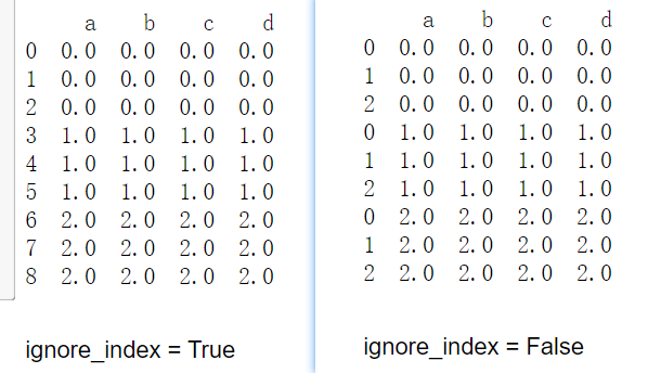
1	res = pd.concat([df1, df2, df3], axis = 0, ignore_index = True) # default don't ignore index, the difference seen in below pic

fig. 1 difference of ignoring index

join = ['inner', 'outer']

import pandas as pd
import numpy as np

df1 = pd.DataFrame(np.ones((3, 4)) * 0, columns = ['a', 'b', 'c', 'd'], index = [1, 2, 3])
df2 = pd.DataFrame(np.ones((3, 4)) * 1, columns = ['b', 'c', 'd', 'e'], index = [0, 1, 2])

# default join is outer, fill the null space with NaN
df3 = pd.concat([df1, df2], axis = 0, join = 'outer', sort=False, ignore_index = True)
# inner will take the intersection index of two arrays
df4 = pd.concat([df1, df2], axis = 0, join = 'inner', sort=False, ignore_index = True)

# 将 df2 合并到 df1，并基于 index 去掉 df2 中有而 df1 没有的数据， 并填充 NaN
df5 = pd.concat([df1, df2], axis = 1, join_axes = [df1.index])

4.2 append

import pandas as pd
import numpy as np

df1 = pd.DataFrame(np.ones((3, 4)) * 0, columns = ['a', 'b', 'c', 'd'])
df2 = pd.DataFrame(np.ones((3, 4)) * 1, columns = ['a', 'b', 'c', 'd'])
df3 = pd.DataFrame(np.ones((3, 4)) * 1, columns = ['a', 'b', 'c', 'd'])

res = df1.append([df2, df3], ignore_index = True)

# add a row series into a df
s1 = pd.Series([1, 2, 3, 4], index = ['a', 'b', 'c', 'd'])
res1 = df1.append(s1, ignore_index = True)

4.3 merge

merged by single key

import pandas as pd
import numpy as np

left = pd.DataFrame({'key': ['K0', 'K1', 'K2', 'K3'],'A': ['A0', 'A1', 'A2', 'A3'],'B': ['B0', 'B1', 'B2', 'B3']})
right = pd.DataFrame({'key': ['K0', 'K1', 'K2', 'K3'],'C': ['C0', 'C1', 'C2', 'C3'],'D': ['D0', 'D1', 'D2', 'D3']})

# merge two dfs based on the same key value
res = pd.merge(left, right, on = 'key')

merged by multiple keys

import pandas as pd
import numpy as np

left = pd.DataFrame({'key1': ['K0', 'K0', 'K1', 'K2'],'key2': ['K0', 'K1', 'K0', 'K1'],'A': ['A0', 'A1', 		'A2', 'A3'],'B': ['B0', 'B1', 'B2', 'B3']})
right = pd.DataFrame({'key1': ['K0', 'K1', 'K1', 'K2'],'key2': ['K0', 'K1', 'K0', 'K0'],'C': ['C0', 'C1', 		'C2', 'C3'],'D': ['D0', 'D1', 'D2', 'D3']})

# merge two dfs based the same key value, default how = inner
res1 = pd.merge(left, right, on = ['key1','key2'])
res2 = pd.merge(left, right, on = ['key1','key2'], how = 'inner')
res2 = pd.merge(left, right, on = ['key1','key2'], indicator = True)

how = ['inner, 'outer','left','right'], if how = 'right', this operation will fill left void space with NaN when left haven't same key value with right, then merge into right.

default indicator is False, this parameter will create a new column named _merge(indicator = 'indicator_column', then the new column's name is indicator_column), which show if both arrays have a meanful value.

merged by index

import pandas as pd
import numpy as np

left = pd.DataFrame({'A': ['A0', 'A1', 'A2', 'A3'],'B': ['B0', 'B1', 'B2', 'B3']}, index = ['K0', 'K1', 'K2','K4'])
right = pd.DataFrame({'C': ['C0', 'C1', 'C2', 'C3'],'D': ['D0', 'D1', 'D2', 'D3']}, index = ['K0', 'K1', 'K3','K5'])
print(left, right, sep = '\n')

# left_index and right_index
res1 = pd.merge(left, right, left_index = True, right_index = True, how = 'inner') # based on left_index = right_index
res2 = pd.merge(left, right, left_index = True, right_index = True, how = 'outer') # fill the blank with NaN

suffixes para

import pandas as pd
import numpy as np

boys = pd.DataFrame({'K': ['K0', 'K1', 'K2','K4'],'age': [11, 23, 32, 12]})
girls = pd.DataFrame({'K': ['K0', 'K1', 'K2','K4'],'age': [14, 43, 12, 22]})

# suffixex means the named methods of same positional column
res = pd.merge(boys, girls, on = 'K', suffixes = ['_boys', '_girls'], how = 'inner')
print(res) #  age_boys  age_girls

5 Read and save file

import pandas as pd

data = pd.read_csv('xx.csv') # read
data.to_csv('xxx.csv') # save file

6 matplotlib

import numpy as np
import pandas as pd
import matplotlib.pyplot as plt
data1 = pd.Series(np.random.randn(1000), index = np.arange(1000))
data2 = pd.DataFrame(np.random.randn(1000, 4), index = np.arange(1000), columns = list('ABCD'))
# print(data1, data2, sep = '\n')
data1 = data1.cumsum()
data2 = data2.cumsum()
# print(data)
data1.plot()
data2.plot()
plt.show()

plot methods

bar, hist, box, kde, area, scatter, hexbin, pie

import numpy as np
import pandas as pd
import matplotlib.pyplot as plt
data = pd.DataFrame(np.random.randn(1000, 4), index = np.arange(1000), columns = list('ABCD'))

data = data.cumsum()

ax = data.plot.scatter(x = 'A', y = 'B',color = 'DarkBlue', label = 'Class1')
data.plot.scatter(x = 'A', y = 'C',color = 'DarkGreen',label = 'Class2',ax = ax)
plt.show()

Result:

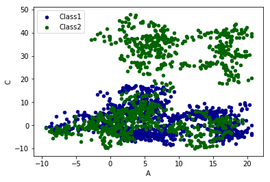
fig. 2 scatter figure

独孤诗人的学习驿站

Pandas

1 Series

1.1 Preparation

1.2 Different data type

1.3 Create DataFrame

1.4 Basic information

1.5 Data type

2 Choose data

2.1 Basic operation

2.2 Index methods

2.3 Conditional operation

2.4 Functional methods

3 DataFrame operation

3.1 Value operation

3.2 Advance operation

3.3 Delete values

4 Merge dataframes

4.1 Concatenation

4.2 append

4.3 merge

5 Read and save file

6 matplotlib